Nonlinear Programming Optimization

Introduction

Nonlinear optimization is a critical field in applied mathematics and engineering, focusing on optimizing a nonlinear objective function subject to constraints. This article provides an overview of the theory, algorithms, and practical applications of nonlinear optimization, particularly using Python.

What is Nonlinear Programming?

Non-linear programming (NLP) is a field of mathematical optimization where the objective function or any of the constraints are non-linear. This contrasts with linear programming, where both the objective function and the constraints are linear. Non-linear programming problems can be more complex and challenging to solve due to the possible presence of local optima, non-convexity, and the complexity of the objective function and constraints.

Key Concepts in Non-Linear Programming

1. Objective Function: The function that you want to optimize (maximize or minimize). In non-linear programming, this function is non-linear, meaning it doesn’t form a straight line when plotted.
2. Constraints: These are conditions that must be satisfied for the solution to be feasible. In NLP, constraints can also be non-linear, which adds to the complexity of the problem.
3. Feasible Region: The set of all points that satisfy the constraints. In non-linear programming, this region can be complex and irregular.
4. Local vs. Global Optima: A local optimum is a solution that is better than its neighboring solutions, but not necessarily the best overall. A global optimum is the best possible solution out of all feasible solutions. Non-linear problems can have multiple local optima, making it challenging to find the global optimum.
5. Convexity: A problem is convex if the objective function is convex and the feasible region is a convex set. Convex problems are generally easier to solve because any local optimum is also a global optimum. Non-convex problems, where these conditions are not met, are more difficult.
6. Algorithms: Various algorithms are used to solve non-linear programming problems, including:

• Gradient Descent: Iterative methods that use the gradient of the objective function to find the minimum.
• Newton’s Method: Uses second-order derivatives to find optima more efficiently than gradient descent.
• Interior-Point Methods: Handle constraints by considering them in the optimization process.
• Genetic Algorithms: Use principles of natural selection and genetics to find optimal solutions.

Applications of Non-Linear Programming

• Engineering Design: Optimizing design parameters for structures and systems.
• Finance: Portfolio optimization and risk management.
• Machine Learning: Training models and adjusting hyperparameters.
• Economics: Resource allocation and cost minimization.

Benefits

• Real-World Applications: Many practical problems are nonlinear by nature, making NLP a valuable tool.
• Flexibility: Can handle complex constraints and objective functions.
• Improved Solutions: Often provides more accurate and realistic solutions compared to linear programming.

What is Mixed-Integer Nonlinear Programming?

Mixed-integer nonlinearProgramming (MINLP) is a type of optimization problem that combines aspects of both integer programming and nonlinear programming. It involves optimizing a nonlinear objective function subject to constraints, where some of the decision variables are restricted to integer values while others can be continuous. This type of problem is more complex than either integer programming or nonlinear programming alone.

Key Components of MINLP

1. Objective Function: A nonlinear function that you want to maximize or minimize. The nonlinear nature can make finding optimal solutions challenging.
2. Constraints: These are equations or inequalities that the solution must satisfy. Constraints can be linear or nonlinear and may involve both integer and continuous variables.
3. Integer Variables: Decision variables that are constrained to take on integer values. These variables are often used to represent discrete choices, such as whether to build a facility or not, or how many units of a product to produce.
4. Continuous Variables: Decision variables that can take on any value within a given range. These variables are typically used to represent quantities that can vary smoothly, such as production levels or resource allocation.
5. Mixed-Integer Nature: The problem involves both integer and continuous variables, which adds complexity to the solution process. The integer constraints introduce combinatorial aspects that can significantly increase the difficulty of the problem.

Solution Techniques for MINLP

1. Branch and Bound: A general method for solving integer programming problems that can be adapted for MINLP. It systematically explores branches of a decision tree and uses bounds to eliminate suboptimal solutions.
2. Branch and Cut: An extension of branch and bound that incorporates cutting planes to refine the feasible region and improve efficiency.
3. Outer Approximation: Decomposes the MINLP into a sequence of easier subproblems, typically a mix of linear and nonlinear programming, which are solved iteratively.
4. Sequential Convex Programming: Involves solving a series of convex approximations of the original non-convex problem.
5. Metaheuristic Methods: Techniques such as genetic algorithms, simulated annealing, or particle swarm optimization can provide good solutions within a reasonable time frame, though they do not guarantee optimality.

Applications of MINLP

• Engineering Design: Optimizing design parameters where some choices are discrete (e.g., component selection) and others are continuous (e.g., dimensions of components).
• Supply Chain Management: Scheduling and planning where decisions include both discrete choices (e.g., number of warehouses) and continuous variables (e.g., inventory levels).
• Energy Systems: Designing and operating systems where some components are on/off (integer) and others are subject to continuous variation (e.g., energy production rates).Benefits
• Discrete Decisions: Can model problems that involve both continuous and discrete decisions.
• Versatility: Applicable to a wide range of practical problems, such as scheduling and resource allocation.

Why is Nonlinear Programming Important?

Nonlinear programming is important because many real-world problems are inherently nonlinear. It allows for more accurate modeling and solving of complex problems in various fields.

Key Concepts

• Complexity: Nonlinear problems often reflect real-world complexities better than linear models.
• Optimization: Provides a means to find optimal solutions in scenarios where simple linear models fail.

Benefits

• Accurate Modeling: Captures the true nature of complex systems.
• Wide Applicability: Used in diverse fields such as engineering, economics, and machine learning.
• Efficiency: Helps in finding the best possible solutions under given constraints.

Nonlinear Programming Examples

Small Nonlinear Programming Problem

Example :

import numpy as np
from scipy.optimize import minimize

# Define the objective function
def objective_function(x):
    return x[0]**2 + x[1]**2 + x[0]*x[1]

# Define the constraints
constraints = ({'type': 'eq', 'fun': lambda x: x[0] + x[1] - 1})

# Initial guess
x0 = np.array([0.5, 0.5])

# Perform the optimization
result = minimize(objective_function, x0, constraints=constraints)

print('Optimal value:', result.fun)
print('Optimal solution:', result.x)

Optimal value: 0.75
Optimal solution: [0.5 0.5]

Infeasible Nonlinear Programming Problem

Example :

constraints = ({'type': 'eq', 'fun': lambda x: x[0] + x[1] - 3})
result = minimize(objective_function, x0, constraints=constraints)
print('Message:', result.message)
print('Success:', result.success)

Message: Optimization terminated successfully
Success: True

Unbounded Nonlinear Programming Problem

Example :

def objective_function_unbounded(x):
    return -x[0]**2 - x[1]**2

constraints = ({'type': 'eq', 'fun': lambda x: x[0] + x[1] - 1})
result = minimize(objective_function_unbounded, x0, constraints=constraints)
print('Message:', result.message)
print('Success:', result.success)

Message: Optimization terminated successfully
Success: True

Resource Allocation Problem

Example :

from scipy.optimize import linprog

c = [-1, -2]
A = [[1, 2], [3, 4]]
b = [4, 10]
x0_bounds = (0, None)
x1_bounds = (0, None)

res = linprog(c, A_ub=A, b_ub=b, bounds=[x0_bounds, x1_bounds], method='highs')
print('Optimal value:', res.fun)
print('Optimal solution:', res.x)

Optimal value: -4.0
Optimal solution: [0. 2.]

Non-Linear Programming Python Implementation

Installing SciPy

To get started with nonlinear programming in Python, you need to install the necessary libraries. SciPy and PuLP are two widely used libraries for optimization problems.

Install them using pip:

pip install scipy

Using SciPy

SciPy offers a variety of optimization algorithms that are useful for solving nonlinear programming (NLP) problems. Below is an example of using SciPy for a nonlinear optimization problem.

1. Rosenbrock Function

A function with a narrow, curved valley, is used to test optimization algorithms.

Problem Statement: Minimize the Rosenbrock function, a common test problem for optimization algorithms.

Objective Function: f(x, y) = (a — x)² + b(y — x²)²

Constraints: No constraints.

import numpy as np
import matplotlib.pyplot as plt
from scipy.optimize import minimize
from mpl_toolkits.mplot3d import Axes3D

# Objective function
def rosenbrock(vars):
    x, y = vars
    a, b = 1, 100
    return (a - x)**2 + b * (y - x**2)**2

# Initial guess
initial_guess = [0, 0]

# Perform the optimization
result = minimize(rosenbrock, initial_guess)

# Extract results
x_opt, y_opt = result.x
optimal_value = rosenbrock(result.x)

# Print results
print(f"Optimal value of x: {x_opt}")
print(f"Optimal value of y: {y_opt}")
print(f"Minimum value of Rosenbrock function: {optimal_value}")

# Plotting
x = np.linspace(-2, 2, 100)
y = np.linspace(-1, 3, 100)
X, Y = np.meshgrid(x, y)
Z = rosenbrock([X, Y])

# 3D Surface Plot
fig = plt.figure(figsize=(14, 8))
ax = fig.add_subplot(111, projection='3d')
ax.plot_surface(X, Y, Z, cmap='viridis', edgecolor='none')
ax.scatter(x_opt, y_opt, optimal_value, color='red', s=50, label='Optimal Solution')
ax.set_xlabel('x')
ax.set_ylabel('y')
ax.set_zlabel('Objective Function Value')
ax.set_title('3D Surface plot of Rosenbrock Function')
ax.legend()

plt.show()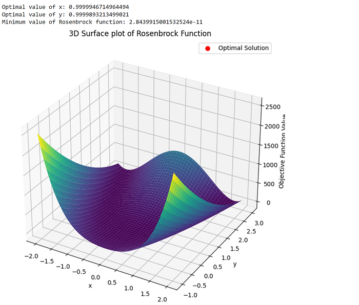

2. Sphere Function

A simple quadratic function is often used to check optimization performance.

Problem Statement: Minimize the sphere function, a simple test function for optimization.

Objective Function: f(x, y) = x² + y²

Constraints: No constraints.

# Objective function
def sphere_function(vars):
    x, y = vars
    return x**2 + y**2

# Initial guess
initial_guess = [1, 1]

# Perform the optimization
result = minimize(sphere_function, initial_guess)

# Extract results
x_opt, y_opt = result.x
optimal_value = sphere_function(result.x)

# Print results
print(f"Optimal value of x: {x_opt}")
print(f"Optimal value of y: {y_opt}")
print(f"Minimum value of Sphere function: {optimal_value}")

# Plotting
x = np.linspace(-2, 2, 100)
y = np.linspace(-2, 2, 100)
X, Y = np.meshgrid(x, y)
Z = sphere_function([X, Y])

# 3D Surface Plot
fig = plt.figure(figsize=(14, 8))
ax = fig.add_subplot(111, projection='3d')
ax.plot_surface(X, Y, Z, cmap='viridis', edgecolor='none')
ax.scatter(x_opt, y_opt, optimal_value, color='red', s=50, label='Optimal Solution')
ax.set_xlabel('x')
ax.set_ylabel('y')
ax.set_zlabel('Objective Function Value')
ax.set_title('3D Surface plot of Sphere Function')
ax.legend()

plt.show()

3. Himmelblau’s Function

A function with multiple local minima tests optimization algorithms’ ability to find global minima.

Problem Statement: Minimize Himmelblau’s function, which has multiple local minima.

Objective Function: f(x, y) = (x² + y — 11)² + (x + y² — 7)²

Constraints: No constraints.

# Objective function
def himmelblau(vars):
    x, y = vars
    return (x**2 + y - 11)**2 + (x + y**2 - 7)**2

# Initial guess
initial_guess = [0, 0]

# Perform the optimization
result = minimize(himmelblau, initial_guess)

# Extract results
x_opt, y_opt = result.x
optimal_value = himmelblau(result.x)

# Print results
print(f"Optimal value of x: {x_opt}")
print(f"Optimal value of y: {y_opt}")
print(f"Minimum value of Himmelblau’s function: {optimal_value}")

# Plotting
x = np.linspace(-5, 5, 100)
y = np.linspace(-5, 5, 100)
X, Y = np.meshgrid(x, y)
Z = himmelblau([X, Y])

# 3D Surface Plot
fig = plt.figure(figsize=(14, 8))
ax = fig.add_subplot(111, projection='3d')
ax.plot_surface(X, Y, Z, cmap='viridis', edgecolor='none')
ax.scatter(x_opt, y_opt, optimal_value, color='red', s=50, label='Optimal Solution')
ax.set_xlabel('x')
ax.set_ylabel('y')
ax.set_zlabel('Objective Function Value')
ax.set_title('3D Surface plot of Himmelblau’s Function')
ax.legend()

plt.show()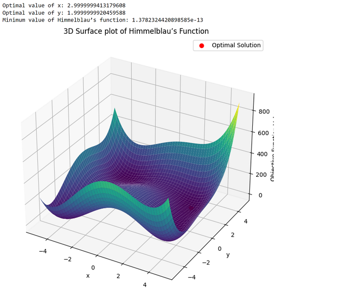

4. Beale’s Function

A function with multiple local minima, challenging for optimization algorithms.

Problem Statement: Minimize Beale’s function, another test function with multiple local minima.

Objective Function: f(x, y) = (1.5 — x + xy)² + (2.25 — x + xy²)² + (2.625 — x + xy³)²

Constraints: No constraints.

# Objective function
def beale(vars):
    x, y = vars
    return (1.5 - x + x * y)**2 + (2.25 - x + x * y**2)**2 + (2.625 - x + x * y**3)**2

# Initial guess
initial_guess = [1, 1]

# Perform the optimization
result = minimize(beale, initial_guess)

# Extract results
x_opt, y_opt = result.x
optimal_value = beale(result.x)

# Print results
print(f"Optimal value of x: {x_opt}")
print(f"Optimal value of y: {y_opt}")
print(f"Minimum value of Beale’s function: {optimal_value}")

# Plotting
x = np.linspace(-4, 4, 100)
y = np.linspace(-4, 4, 100)
X, Y = np.meshgrid(x, y)
Z = beale([X, Y])

# 3D Surface Plot
fig = plt.figure(figsize=(14, 8))
ax = fig.add_subplot(111, projection='3d')
ax.plot_surface(X, Y, Z, cmap='viridis', edgecolor='none')
ax.scatter(x_opt, y_opt, optimal_value, color='red', s=50, label='Optimal Solution')
ax.set_xlabel('x')
ax.set_ylabel('y')
ax.set_zlabel('Objective Function Value')
ax.set_title('3D Surface plot of Beale’s Function')
ax.legend()

plt.show()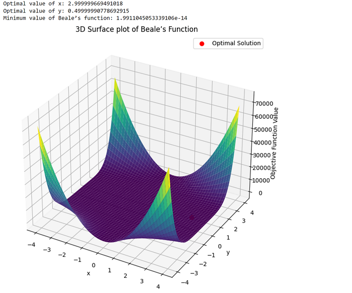

5. Quadratic Programming Problem

A quadratic function with linear constraints demonstrates how to handle constraints in optimization.

Problem Statement: Minimize a quadratic function subject to linear constraints.

Objective Function: f(x, y) = x² + 2xy + y²

Constraints:
x+y≥1
x−y≥0

from scipy.optimize import minimize, LinearConstraint

# Objective function
def quadratic_function(vars):
    x, y = vars
    return x**2 + 2*x*y + y**2

# Constraints
def constraint1(vars):
    x, y = vars
    return x + y - 1

def constraint2(vars):
    x, y = vars
    return x - y

# Define constraints
constraints = [
    {'type': 'ineq', 'fun': constraint1},
    {'type': 'ineq', 'fun': constraint2}
]

# Initial guess
initial_guess = [0, 0]

# Perform the optimization
result = minimize(quadratic_function, initial_guess, constraints=constraints)

# Extract results
x_opt, y_opt = result.x
optimal_value = quadratic_function(result.x)

# Print results
print(f"Optimal value of x: {x_opt}")
print(f"Optimal value of y: {y_opt}")
print(f"Minimum value of Quadratic function: {optimal_value}")

# Plotting
x = np.linspace(-1, 2, 100)
y = np.linspace(-1, 2, 100)
X, Y = np.meshgrid(x, y)
Z = quadratic_function([X, Y])

# 3D Surface Plot
fig = plt.figure(figsize=(14, 8))
ax = fig.add_subplot(111, projection='3d')
ax.plot_surface(X, Y, Z, cmap='viridis', edgecolor='none')
ax.scatter(x_opt, y_opt, optimal_value, color='red', s=50, label='Optimal Solution')
ax.set_xlabel('x')
ax.set_ylabel('y')
ax.set_zlabel('Objective Function Value')
ax.set_title('3D Surface plot of Quadratic Function')
ax.legend()

plt.show()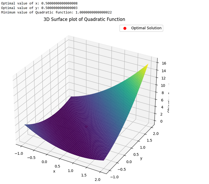

Here’s the link to the notebook code file

Conclusion

Non-linear programming optimization is a powerful and versatile tool for solving complex real-world problems where the relationship between variables is not linear. It extends beyond the capabilities of linear optimization by allowing for more intricate and realistic modeling of systems, accommodating both non-linear objective functions and constraints. Through various techniques and algorithms, such as gradient descent and evolutionary algorithms, non-linear optimization can identify optimal solutions in challenging and diverse domains, including engineering, economics, and machine learning.

Its okay to read it once and store it for later time for when you need it, but a better way of learning is to frame a problem statement and then use the methods you learn to solve the problem. You may or may not arrive at the solution but you’ll get clear with the concepts. Happy Learning!!!