Backtesting-02

6 min readJan 17, 2024

Examples Of Backtesting

In this segment, we present a straightforward Python implementation of backtesting, utilizing the historical dataset obtained from yfinance. This is an extension of the previous part and here we are going to calculate a couple of more stats which are considered for backtesting. Overall in this part we will be creating a framework for the entire process.

Let’s start by importing the necessary libraries.

import yfinance as yf
import pandas as pd
from datetime import datetime
import numpy as np
from tabulate import tabulate
import warnings
warnings. simplefilter(action='ignore', category=Warning)

Data Download by using yfinance:

# Set the ticker symbol for Nifty 50
nifty_symbol = "RELIANCE.BO"

# Set the start date for the historical data
start_date = "2010-01-01"  # Adjusted to the previous Friday

# Set the end date to the current date
end_date = datetime.today().strftime('%Y-%m-%d')

# Download historical data
nifty_data = yf.download(nifty_symbol, start=start_date, end=end_date)

# Print the historical data with returns, weekly returns, monthly returns, and day of the week
print(nifty_data.tail(100))

# Save the data to a CSV file
nifty_data.to_csv('RELIANCE.csv')

Create a function named `GoldenCrossoverSignal` that computes the 20-day and 50-day Simple Moving Averages (sma20 and sma50) along with buy and sell signals:

def GoldenCrossoverSignal(name):
    path = f'RELIANCE.csv'
    data = pd.read_csv(path, parse_dates=['Date'], index_col='Date')
    data['Prev_Close'] = data.Close.shift(1)
    data['20_sma'] = data.Prev_Close.rolling(window=20, min_periods=1).mean()
    data['50_sma'] = data.Prev_Close.rolling(window=50, min_periods=1).mean()
    data['Signal'] = 0
    data['Signal'] = np.where(data['20_sma'] > data['50_sma'], 1, 0)
    data['Position'] = data.Signal.diff()

    
    df_pos = data[(data['Position'] == 1) | (data['Position'] == -1)].copy()
    df_pos['Position'] = df_pos['Position'].apply(lambda x: 'Buy' if x == 1 else 'Sell')

    return df_pos

Execute the function:

data=GoldenCrossoverSignal('RELIANCE')
data

Extracting Trading Signals: Creating a DataFrame for Buy and Sell Positions:

required_df = data[(data.index >= data[data['Position'] == 'Buy'].index[0]) & (data.index <= data[data['Position'] == 'Sell'].index[-1])]
required_df

The code snippet extracts a subset of the data DataFrame, focusing only on the rows where the 'Position' column is labeled as 'Buy.' The resulting required_df contains data from the first 'Buy' signal to the last 'Sell' signal in the original dataset.

saves the DataFrame required_df to a CSV file with the specified file path:

required_df.to_csv(f'rel_required.csv')

Algorithmic Trading Strategy Backtesting and Performance Analysis:

# Name, Entry TIme, Entry PRice, QTY, Exit Time, Exit Price
class Backtest:
    def __init__(self):
        self.columns = ['Equity Name', 'Trade', 'Entry Time', 'Entry Price', 'Exit Time', 'Exit Price', 'Quantity', 'Position Size', 'PNL', '% PNL']
        self.backtesting = pd.DataFrame(columns=self.columns)

    def buy(self, equity_name, entry_time, entry_price, qty):
        self.trade_log = dict(zip(self.columns, [None] * len(self.columns)))
        self.trade_log['Trade'] = 'Long Open'
        self.trade_log['Quantity'] = qty
        self.trade_log['Position Size'] = round(self.trade_log['Quantity'] * entry_price, 3)
        self.trade_log['Equity Name'] = equity_name
        self.trade_log['Entry Time'] = entry_time
        self.trade_log['Entry Price'] = round(entry_price, 2)
    def sell(self, exit_time, exit_price, exit_type, charge):
        self.trade_log['Trade'] = 'Long Closed'
        self.trade_log['Exit Time'] = exit_time
        self.trade_log['Exit Price'] = round(exit_price, 2)
        self.trade_log['Exit Type'] = exit_type
        self.trade_log['PNL'] = round((self.trade_log['Exit Price'] - self.trade_log['Entry Price']) * self.trade_log['Quantity'] - charge, 3)
        self.trade_log['% PNL'] = round((self.trade_log['PNL'] / self.trade_log['Position Size']) * 100, 3)
        self.trade_log['Holding Period'] = exit_time - self.trade_log['Entry Time']
        self.backtesting = self.backtesting._append(self.trade_log, ignore_index=True)
    def stats(self):
        df = self.backtesting
        parameters = ['Total Trade Scripts', 'Total Trade', 'PNL',  'Winners', 'Losers', 'Win Ratio','Total Profit', 'Total Loss', 'Average Loss per Trade', 'Average Profit per Trade', 'Average PNL Per Trade', 'Risk Reward']
        total_traded_scripts = len(df['Equity Name'].unique())
        total_trade = len(df.index)
        pnl = df.PNL.sum()
        winners = len(df[df.PNL > 0])
        loosers = len(df[df.PNL <= 0])
        win_ratio = str(round((winners/total_trade) * 100, 2)) + '%'
        total_profit = round(df[df.PNL > 0].PNL.sum(), 2)
        total_loss  = round(df[df.PNL <= 0].PNL.sum(), 2)
        average_loss_per_trade = round(total_loss/loosers, 2)
        average_profit_per_trade = round(total_profit/winners, 2)
        average_pnl_per_trade = round(pnl/total_trade, 2)
        risk_reward = f'1:{-1 * round(average_profit_per_trade/average_loss_per_trade, 2)}'
        data_points = [total_traded_scripts,total_trade,pnl,winners, loosers, win_ratio, total_profit, total_loss, average_loss_per_trade, average_profit_per_trade, average_pnl_per_trade, risk_reward]
        data = list(zip(parameters,data_points ))
        print(tabulate(data, ['Parameters', 'Values'], tablefmt='psql'))

Explore the implementation of a comprehensive algorithmic trading strategy backtesting framework using Python. This project covers recording buy and sell transactions, calculating profits and losses, and generating key performance metrics for data-driven analysis.

Key Features:

Simulate trading strategies with entry and exit points.
Record trade details, including entry and exit times, prices, quantities, and more.
Analyze trading performance with statistics such as total trades, P&L, win ratio, and risk-reward ratio.
Visualize and interpret the results for effective strategy evaluation.

Capital Allocation and Trade Iteration:

bt = Backtest()
capital = 50000
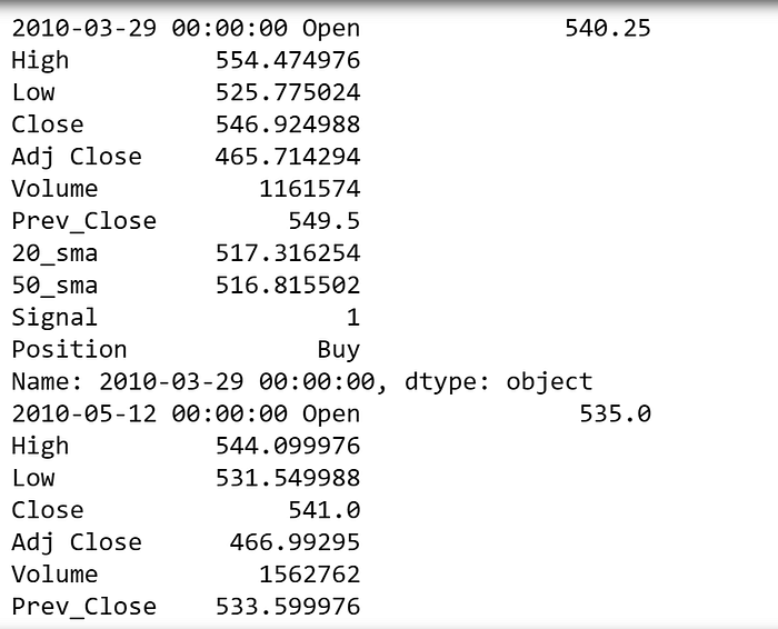
for index, data in required_df.iterrows():
    print(index, data)

It prepares for backtesting a trading strategy with a specified initial capital and prints the index and data for each iteration.

Algorithmic Trading Backtesting with Dynamic Capital Allocation:

bt = Backtest()
capital = 50000
for index, data in required_df.iterrows():
    if(data.Position == 'Buy'):
        qty = capital // data.Open
        bt.buy('RELIANCE', index, data.Open, qty)
    elif data.Position == 'Sell':
        bt.sell(index, data.Open, 'Exit Trigger', 0)

Explore a Python-based algorithmic trading backtesting implementation where a Backtest class is utilized to simulate buy and sell signals. The strategy dynamically allocates capital for buying and triggers sell orders based on predefined signals. This article provides insights into the hands-on application of backtesting strategies and dynamically managing capital for optimal trading simulations.

bt.backtesting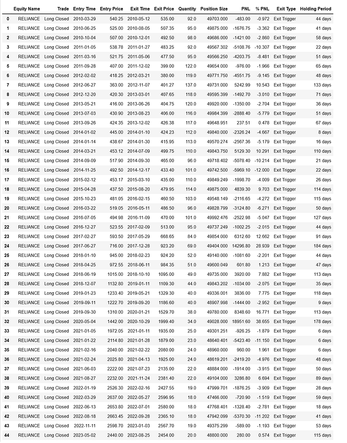

The entry time was generated for each buy signal, and the exit time was generated for each sell signal.

Trades for specific equity (RELIANCE) by indicating whether the trade was a long position closure, the entry and exit times, prices, quantity, position size, profit and loss (PNL), percentage PNL, exit type, and the holding period.

saves the DataFrame bt.backtesting to a CSV file with the specified file path:

bt.backtesting.to_csv(f'rel_pnl.csv')

Unveiling Key Metrics with Backtest Statistics:

bt.stats()

The bt.stats() method is designed to generate and display statistical metrics based on the trading transactions recorded in the backtesting process. This method calculates various performance indicators that provide insights into the effectiveness of the algorithmic trading strategy. The statistics typically include metrics such as the total number of trades, total profit and loss (PNL), win ratio, average profit per trade, average loss per trade, and risk-reward ratio.

In the given code, the stats() method prints a tabulated summary containing important statistics for the backtesting results. The displayed metrics include:

Total Trade Scripts
Total Trade
PNL (Total Profit and Loss)
Winners (Number of Profitable Trades)
Losers (Number of Losing Trades)
Win Ratio
Total Profit
Total Loss
Average Loss per Trade
Average Profit per Trade
Average PNL per Trade
Risk-Reward Ratio

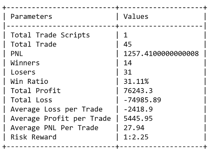
sum of pnl:

bt.backtesting.PNL.sum()

Conclusion:

As we have seen, it is not only the final cumulative profit that we need to see while we analyze backtest results. We need to see the volatility of the profits as well. Now here are certain challenges to the system which we are going to address in the upcoming series.

Is the 20–50 crossover optimum
Is the result overfitted (How does it perform on out-sample data)
What is the drawdown and losing streak (This is critical question)

I highly suggest you to follow the series in orderly manner. In case you have any questions related to this or any other topic of interest, feel free to shoot me a question at Topmate

You can follow me anywhere you wish for receiving updates about my journey and projects.

Website

Happy Learning !!!

Backtesting-02

Examples Of Backtesting

Conclusion:

Written by Gaurav Kumar